Protein-ligand binding in a membrane¶

This example calculates the binding free energy of ubiquinone (UQ2) to a membrane protein (PROA). The source system was prepared with CHARMM-GUI and contains an explicit DOPC/POPC bilayer, solvent, and ions. The calculation uses a heterogeneous implicit-membrane PB model.

Protocol

Single trajectory
Force field

CHARMM
Membrane model

Heterogeneous PB (memopt=2)
Bundled test

gmx_MMPBSA_test -t 6

Representative system

This membrane protein-ligand complex demonstrates the heterogeneous implicit-membrane PB workflow for a CHARMM topology. CHARMM support is not limited to this molecular composition, but implicit-membrane calculations require compatible membrane geometry and method-specific settings.

CHARMM CMAP conversion

The current GROMACS-to-AMBER topology conversion omits CHARMM CMAP terms and reports this during setup. The example exercises the complete implicit-membrane workflow, but quantitative CHARMM applications should assess the effect of the missing CMAP contribution before interpreting binding energies.

CHARMM PB radii

PBRadii=7 selects the charmm_radii set, which is intended only for systems prepared with CHARMM force fields. Its protein radii draw on work by Nina, Belogv, and Roux, nucleic-acid radii on Banavali and Roux, and additional elements on Fortuna and Costa. With radiopt=0, PBSA uses these radii from the generated AMBER topologies.

Before you begin¶

The manual workflow uses the following files and selections:

Calculation settings

mmpbsa.in (-i)
GROMACS system

Structure com.pdb (-cs) and topology topol.top (-cp). Keep the toppar directory containing the referenced CHARMM *.itp files beside topol.top.
Trajectory

Fitted four-frame trajectory md.xtc (-ct), with the membrane normal aligned to the z axis
Molecular selections

Index index.ndx (-ci) with receptor PROA and ligand UQ2 (-cg)

The complete structure contains 95,472 atoms: protein, ligand, DOPC/POPC lipids, ions, and TIP3 water. The selected binding system contains the 2,985-atom receptor and 49-atom ligand. See the complete command-line reference for all options.

Run the example¶

Run the bundled test¶

The quickest way to reproduce this example is through the test runner:

gmx_MMPBSA_test -t 6

This is a slow test because PB calculations are performed for a membrane protein. See the gmx_MMPBSA_test documentation for download, selection, and cleanup options.

Run it manually¶

Download the protein-membrane example as a ZIP archive.

Extract the archive, change to the Protein_membrane directory, and choose either the serial or MPI command. You can also view the example files on GitHub before downloading them.

SerialWith MPI

gmx_MMPBSA -O \
  -i mmpbsa.in \
  -cs com.pdb \
  -ct md.xtc \
  -ci index.ndx \
  -cg PROA UQ2 \
  -cp topol.top \
  -o FINAL_RESULTS_MMPBSA.dat \
  -eo FINAL_RESULTS_MMPBSA.csv

mpirun -np 2 gmx_MMPBSA -O \
  -i mmpbsa.in \
  -cs com.pdb \
  -ct md.xtc \
  -ci index.ndx \
  -cg PROA UQ2 \
  -cp topol.top \
  -o FINAL_RESULTS_MMPBSA.dat \
  -eo FINAL_RESULTS_MMPBSA.csv

Configure the calculation¶

The example uses the concise mmpbsa.in shown first below. The all-options version was generated with gmx_MMPBSA --create_input pb_mem and then adapted with the same example-specific values. The concise block is the runnable starting point; the generated block includes additional options and defaults, so the two blocks are not textually identical. Both blocks therefore describe the same implicit-membrane PB calculation.

Concise inputGenerated input - all options

mmpbsa.in
Sample input file for MMPBSA with membrane proteins
# This input provides a practical starting point for implicit-membrane PB calculations.
# Review the membrane geometry, dielectric model, and PB settings for your system.

&general
sys_name="Prot-Memb-PROA-UQ2",
startframe=1,
endframe=4,
PBRadii=7,
/
&pb
memopt=2, emem=7.0, indi=1.0,
mctrdz=automatic, mthick=automatic, membrane_atoms="P", poretype=1,
radiopt=0, istrng=0.150, fillratio=1.25, inp=2,
sasopt=0, solvopt=2, ipb=1, bcopt=10, nfocus=1, linit=1000,
eneopt=1, cutfd=7.0, cutnb=99.0,
maxarcdot=15000,
npbverb=1,
/

mmpbsa.in generated with --create_input pb_mem
Input block generated for the 1.7.0 release.
Be careful with the variables you modify, some can have severe consequences on the results you obtain.

# General namelist variables
&general
  sys_name                       = "Prot-Memb-PROA-UQ2"                   # System name; e.g. "complex"
  startframe                     = 1                                      # First frame; e.g. 1
  endframe                       = 4                                      # Last frame; e.g. 100
  interval                       = 1                                      # Frame interval; e.g. 1


  PBRadii                        = 7                                      # PB radii set; 1-7
  temperature                    = 298.15                                 # Temperature (K); e.g. 298.15
  qh_entropy                     = 0                                      # Legacy QH output reader; new calculations reject 1
  interaction_entropy            = 0                                      # Run IE entropy; 0/1
  ie_segment                     = 25                                     # IE tail diagnostic only (%); not primary IE; e.g. 25
  c2_entropy                     = 0                                      # Run C2 entropy; 0/1
  assign_chainID                 = 0                                      # Assign chain IDs; 0/1
  exp_ki                         = 0.0                                    # Experimental Ki (nM); e.g. 0.0
  full_traj                      = 0                                      # Write full trajectory; 0/1
  gmx_path                       = ""                                     # GROMACS path; e.g. "/usr/bin"
  keep_files                     = 2                                      # Files to keep; 0-2
  netcdf                         = 0                                      # Use NetCDF; 0/1
  solvated_trajectory            = 1                                      # Clean solvated traj.; 0/1
  explicit_waters                = 0                                      # Explicit waters; e.g. 10
  explicit_waters_mask           = "dASA"                                     # Water reference; e.g. ":1-10", "within 4", "dASA"
  explicit_waters_group          = "automatic"                                     # Solvent group; e.g. "TIP3" or "automatic"
  explicit_waters_dasa_cutoff    = 0.5                                    # dASA cutoff; e.g. 0.5
  explicit_waters_as             = "receptor"                             # Water owner; e.g. "receptor"
  explicit_waters_extra_points   = "error"                                # Virtual sites; "error" or "strip"
  verbose                        = 1                                      # Output verbosity; 0-2
/

# (AMBER) Poisson-Boltzmann namelist variables
&pb
  ipb                            = 1                                      # PB model; e.g. 2
  inp                            = 2                                      # Nonpolar method; 1 or 2
  indi                           = 1.0                                    # Internal dielectric; e.g. 1.0
  exdi                           = 78.5                                   # External dielectric; e.g. 78.5
  emem                           = 7.0                                    # Membrane dielectric; e.g. 4.0
  smoothopt                      = 1                                      # Dielectric smoothing; 0-2
  istrng                         = 0.150                                  # Ionic strength (M); e.g. 0.150
  radiopt                        = 0                                      # Use optimized radii; 0/1
  prbrad                         = 1.4                                    # Probe radius (A); e.g. 1.4
  iprob                          = 2.0                                    # Ion probe (A); e.g. 2.0
  sasopt                         = 0                                      # PB surface option; 0/1
  arcres                         = 0.25                                   # Arc resolution (A); e.g. 0.25
  memopt                         = 2                                      # Use membrane PB; 0-3
  mprob                          = 2.7                                    # Membrane probe (A); e.g. 2.7
  mthick                         = "automatic"                            # Membrane thickness (A), or automatic
  mctrdz                         = "automatic"                            # Membrane Z offset (A), or automatic
  membrane_atoms                 = "P"                                    # Atom names for automatic membrane parameters; semicolon-separated
  poretype                       = 1                                      # Pore type; 1 or 2
  npbopt                         = 0                                      # Use nonlinear PB; 0/1
  solvopt                        = 2                                      # PB solver; e.g. 1
  accept                         = 0.001                                  # Convergence; e.g. 0.001
  linit                          = 1000                                   # SCF iterations; e.g. 1000
  fillratio                      = 1.25                                   # Grid fill ratio; e.g. 4
  scale                          = 2.0                                    # Grid scale; e.g. 2
  nbuffer                        = 0.0                                    # Grid buffer; e.g. 0
  nfocus                         = 1                                      # Focus levels; e.g. 2
  fscale                         = 8                                      # Focus scale; e.g. 8
  npbgrid                        = 1                                      # Grid update freq.; e.g. 1
  bcopt                          = 10                                     # Boundary condition; e.g. 5
  eneopt                         = 1                                      # Energy option; e.g. 2
  frcopt                         = 0                                      # Force output; e.g. 0
  scalec                         = 0                                      # Reaction field option; e.g. 0
  cutfd                          = 7.0                                    # FD cutoff (A); e.g. 5
  cutnb                          = 99.0                                   # Nonbonded cutoff (A); e.g. 0
  nsnba                          = 1                                      # Pairlist frequency; e.g. 1
  decompopt                      = 2                                      # Decomp scheme; 1 or 2
  use_rmin                       = 1                                      # Use Rmin radii; 0/1
  sprob                          = 0.557                                  # SASA probe (A); e.g. 0.557
  vprob                          = 1.3                                    # Volume probe (A); e.g. 1.3
  rhow_effect                    = 1.129                                  # Water density; e.g. 1.129
  use_sav                        = 1                                      # Use SAV cavity; 0/1
  cavity_surften                 = 0.0378                                 # Cavity surften; e.g. 0.0378
  cavity_offset                  = -0.5692                                # Cavity offset; e.g. -0.5692
  maxsph                         = 400                                    # Max surface dots; e.g. 400
  maxarcdot                      = 15000                                  # Max arc dots; e.g. 1500
  npbverb                        = 1                                      # PB verbosity; 0/1
/

Keep in mind

This input provides a practical starting point for implicit-membrane PB calculations. Review membrane placement, dielectric treatment, PB radii, grid convergence, sampling, and the CMAP limitation for the intended system. Additional input-file options may be needed for a production protocol.

How this example works¶

The ST approximation extracts PROA and UQ2 from the same four trajectory frames. The explicit DOPC/POPC bilayer, ions, and water remain available in the full source structure and trajectory but are not retained in the final complex, receptor, or ligand calculation topologies. The unstripped trajectory is used to resolve the implicit membrane geometry before the selected solute trajectory is prepared.

PBRadii=7 assigns CHARMM-specific radii during topology conversion. The CHARMM bonded and nonbonded parameters are read from the topology include tree. CMAP terms are the stated exception.

Automatic membrane placement¶

mctrdz=automatic, mthick=automatic, and membrane_atoms="P" use lipid phosphorus atoms from the original trajectory to determine the bilayer center and leaflet separation. For the bundled four frames, the calculation resolves a center of approximately 62.316 Å and a thickness of 37.3 Å.

The membrane normal must already be aligned with z, and the trajectory should be continuous across periodic boundaries. Automatic detection does not reorient or unwrap the trajectory. Numeric center and thickness values can be supplied independently when a fixed placement is preferred.

The calculation retains two diagnostics:

GMXMMPBSA_membrane_parameters.csv: per-frame membrane centers, thicknesses, and resolved values.
GMXMMPBSA_membrane_parameters.png: phosphorus distributions, leaflet assignments, and slab boundaries.

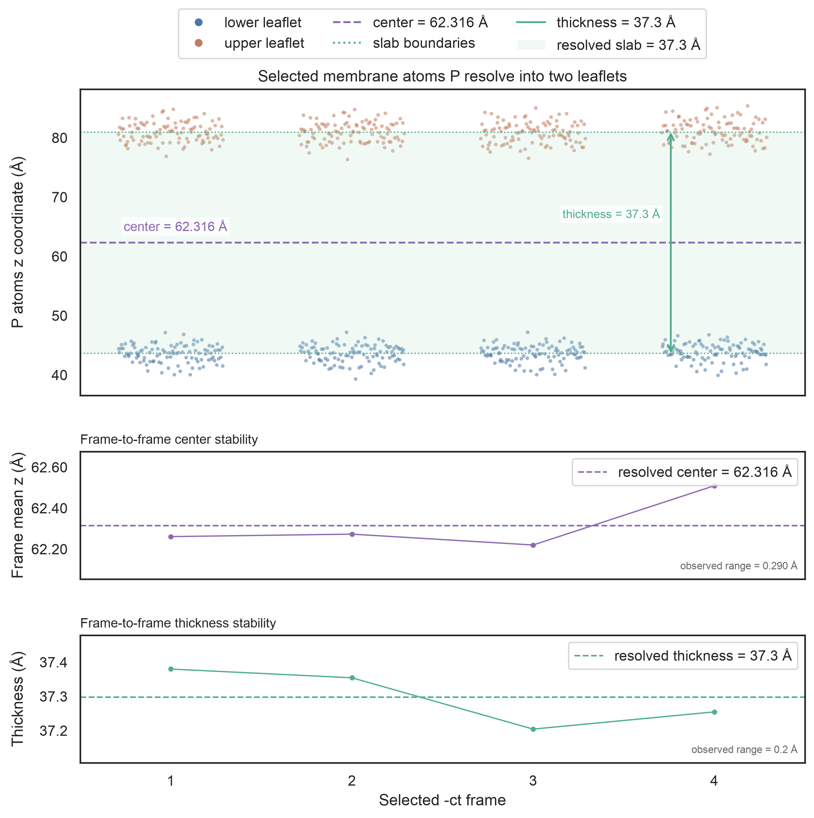
Automatic membrane center and thickness diagnostics

Implicit-membrane PB settings¶

memopt=2 selects the heterogeneous dielectric profile fitted with PCHIP, while poretype=1 enables automatic pore detection. See the heterogeneous implicit-membrane model for the method and model assessment.

The calculation uses the linear PB equation with periodic boundary conditions (ipb=1, bcopt=10) and the geometric multigrid solver (solvopt=2). sasopt=0 uses the solvent-excluded surface, and eneopt=1 selects the P3M total electrostatic-energy treatment required by this periodic setup (this is not NLPB: npbopt=0). The nonzero cutnb=99.0 is the van der Waals cutoff used with eneopt=1; cutfd=7.0 controls the finite-difference direct-sum cutoff.

With eneopt=1, the PB reaction-field and Coulombic contributions are combined in EEL, while EPB is reported as zero - the same Amber P3M bookkeeping as for NLPB. Consequently, the separately labeled gas and solvation subtotals (ΔGGAS / ΔGSOLV) should not be interpreted as the usual MM/PBSA partition; ΔTOTAL retains the solver's complete electrostatic contribution. See eneopt. Periodic PB methods for membrane MMPBSA are discussed in the corresponding implementation study.

The reduced fillratio=1.25 keeps this example's memory requirements manageable. Increasing it enlarges the finite-difference grid and can substantially increase RAM use, particularly with multiple MPI ranks. Grid and solver convergence should be checked before quantitative application.

Expected outputs¶

A successful calculation produces:

FINAL_RESULTS_MMPBSA.dat: the implicit-membrane MM/PBSA summary and binding-energy statistics.
FINAL_RESULTS_MMPBSA.csv: the per-frame energy terms requested with -eo.
The CSV and PNG membrane-placement diagnostics described above.

Analyze the results¶

Open the result with gmx_MMPBSA_ana for interactive inspection and plotting. Remember that EEL contains the combined electrostatic contribution for this eneopt=1 calculation. See the gmx_MMPBSA_ana documentation for usage details.

Last update: September 13, 2026 05:57:32
Created: October 17, 2020 22:35:03