The input file¶

Description¶

gmx_MMPBSA input file contains all the specifications for the calculations. The input file is syntactically similar to other programs in Amber, although we incorporated a new format more similar to the one used on GROMACS *.mdp files (see bleow). The input file contains sections called namelist where the variables are defined for each calculation. The allowed namelists are:

• &general: contains variables that apply to all aspects of the calculation or parameters required for building AMBER topologies from GROMACS files.
• &gb: unique variables to Generalized Born (GB) calculations.
• &gbnsr6: unique variables to GBNSR6 calculations.
• &pb: unique variables to Poisson Boltzmann (PB) calculations.
• &rism: unique variables to 3D-RISM calculations.
• &alanine_scanning: unique variables to alanine scanning calculations.
• &decomp: unique variables to the decomposition scheme.
• &nmode: unique variables to the normal mode (NMODE) calculations used to approximate vibrational entropies.

Generation of input files with gmx_MMPBSA¶

The input file can be created using gmx_MMPBSA by selecting the calculations you want to perform.

gmx_MMPBSA --create_input args

where `args` can be:  gb, gbnsr6, pb, rism, ala, decomp, nmode, all

Example:

gmx_MMPBSA --create_input gb

gmx_MMPBSA --create_input pb

gmx_MMPBSA --create_input gb pb decomp

gmx_MMPBSA --create_input

gmx_MMPBSA --create_input all

Implemented in v1.5.0

Format¶

All the input variables are described below according to their respective namelists. Descriptions are taken from original sources and modified accordingly when needed. Integers and floating point variables should be typed as-is while strings should be put in either single- or double-quotes. All variables should be set with variable = value and separated by commas is they appear in the same line. If the variables appear in different lines, the comma is no longer needed. See several examples are shown below. As you will see, several calculations can be performed in the same run (i.e. &gb and &pb; &gb and &alanine_scanning; &pb and &decomp; etc). As we have mentioned, the input file can be generated using the create_input option of gmx_MMPBSA. This style, while retaining the same Amber format (derived from Fortran), is aesthetically more familiar to the GROMACS style (*.mdp). However, it maintains the same essence, so it could be defined in any of the two format styles or even combined. See the formats below:

# General namelist variables
&general
  sys_name             = ""                      # System name
  startframe           = 1                       # First frame to analyze
  endframe             = 9999999                 # Last frame to analyze
  ...
  interval              = 1                      # The offset from which to choose frames from each trajectory file
/

# Generalized-Born namelist variables
&gb
  igb                  = 5                       # GB model to use
  ...
  probe                = 1.4                     # Solvent probe radius for surface area calc
/

# General namelist variables
&general
  sys_name = "", startframe = 1, endframe = 9999999
  ...
  interval = 1
/

# Generalized-Born namelist variables
&gb
  igb = 5, 
  ...
  probe = 1.4
/

Namelists¶

&general namelist variables¶

Basic input options¶

sys_name (Default = None)

Define the System Name. This is useful when trying to analyze several systems at the same time or calculating the correlation between the predicted and the experimental energies. If the name is not defined, one will be assigned when loading the system in gmx_MMPBSA_ana on a first-come, first-served basis.

Tip

The definition of the system name is entirely optional, however it can provide a better clarity during the results analysis. All files associated with this system will be saved using its name.

Implemented in v1.4.0

startframe (Default = 1)

The frame from which to begin extracting snapshots from the full, concatenated trajectory comprised of every trajectory file placed on the command-line. This is always the first frame read.

endframe (Default = 9999999)

The frame from which to stop extracting snapshots from the full, concatenated trajectory comprised of every trajectory file supplied on the command-line.

interval (Default = 1)

The offset from which to choose frames from each trajectory file. For example, an interval of 2 will pull every 2^nd frame beginning at startframe and ending less than or equal to endframe.

Parameter options¶

forcefields (Default = "oldff/leaprc.ff99SB,leaprc.gaff")

Comma-separated list of force fields used to build Amber topologies. This variable is more flexible than the previous ones (protein_forcefield and ligand_forcefield). The goal of this variable is to provide convenient support for complex systems with several components. It supports all force fields tested in previous protein_forcefield and ligand_forcefield variables.

Tip

• The value of this variable depends on the force field you used for your system in GROMACS
• You don't need to define forcefields` variable when you using a topology. Please refer to the section "How gmx_MMPBSA works"
• The notation format is the one used in tleap
• In general, any forcefield present in $AMBERHOME/dat/leap/cmd could be use with forcefields variable. (Check §3 for more information)
• Be cautious when defining this variable since you can define two forces fields with a similar purpose which can generate inconsistencies.

Input files samples:

Protein and/or Nucleic acidsProtein onlyProtein + DNAProtein + RNA + Organic mol.

Input file with forcefield variable defined for a system with protein and/or nucleic acids

&general
forcefields="oldff/leaprc.ff99SB" 
/

Input file with forcefield variable defined for a system with only protein

&general
forcefields="leaprc.protein.ff14SB" 
/

Input file with forcefield variable defined for a system with protein and nucleic acids (DNA)

&general
forcefields="leaprc.protein.ff14SB,leaprc.DNA.bsc1" 
/

Input file with forcefield variable defined for a system with protein, nucleic acids (RNA) and a organic molecule

&general
forcefields="leaprc.protein.ff14SB,leaprc.RNA.OL3,leaprc.gaff2" 
/

Forcefields for Protein/Nucleic Acids

Name	Description
"oldff/leaprc.ff99"	ff99 for proteins and nucleic acids
"oldff/leaprc.ff03"	ff03 (Duan et al.) for proteins and nucleic acids
"oldff/leaprc.ff99SB"	ff99SB for proteins and nucleic acids
"oldff/leaprc.ff99SBildn"	ff99SB modified for the "ILDN" changes for proteins and nucleic acids
"oldff/leaprc.ff99bsc0"	ff99SB force field using parmbsc0 for nucleic acid

Forcefields only for proteins

Name	Description
"leaprc.protein.ff14SB"	ff14SB only for proteins
"leaprc.protein.ff19SB"	ff19SB only for proteins

Forcefields only for Nucleic Acids

Name	Description
"leaprc.DNA.bsc1"	ff99bsc0+bsc1 only for DNA
"leaprc.DNA.OL15"	ff99bsc0+OL15 only for DNA
"leaprc.RNA.OL3"	ff99bsc0_chiOL3 only for RNA

Forcefields for organic molecules, glycans and zwitterionic amino acids

Name	Description
"leaprc.gaff"	General Amber Force Field for organic molecules
"leaprc.gaff2"	General Amber Force Field 2 for organic molecules
"leaprc.GLYCAM_06j-1"	Glycam_06j-1 carbohydrate ff (Compatible with ff12SB and later)
"leaprc.GLYCAM_06EPb"	GLYCAM-06EPb carbohydrate ff (Compatible with ff12SB and later)
"gmxMMPBSA/leaprc.GLYCAM_06h-1"	* GLYCAM-0606h-1 carbohydrate ff (Compatible with ff99SB and earlier)
"gmxMMPBSA/leaprc.zaa99SB"	* Force field for Zwitterionic amino acids (Compatible with ff99SB)

Tip

* We added the gmxMMPBSA data to the tleap path. This way, we keep gmx_MMPBSA data separated from Amber's.

Implemented in v1.4.1

Modified in v1.4.3: Internal change

Updated in v1.5.0: Documentation updated

protein_forcefield

Define the force field to build Amber topology for protein

Removed in v1.5.0: Use forcefields variable

ligand_forcefield

Define the force field to build Amber topology for ligand (small molecule)

Removed in v1.5.0: Use forcefields variable

ions_parameters (Default = 1)

Define ions parameters to build the Amber topology (see §3.6).

• 1: frcmod.ions234lm_126_tip3p (Li/Merz ion parameters for +2 to +4 ions in TIP3P water (12-6 normal usage set))
• 2: frcmod.ions234lm_126_spce (same, but in SPC/E water)
• 3: frcmod.ions234lm_126_tip4pew (same, but in TIP4P/EW water)
• 4: frcmod.ions234lm_hfe_tip3p (Li/Merz ion parameters for +2 to +4 ions in TIP3P water (12-6 HFE set))
• 5: frcmod.ions234lm_hfe_spce (same, but in SPC/E water)
• 6: frcmod.ions234lm_hfe_tip4pew (same, but in TIP4P/EW water)
• 7: frcmod.ions234lm_iod_tip3p (Li/Merz ion parameters for +2 to +4 ions in TIP3P water (12-6 IOD set))
• 8: frcmod.ions234lm_iod_spce (same, but in SPC/E water)
• 9: frcmod.ions234lm_iod_tip4pew (same, but in TIP4P/EW water)
• 10: frcmod.ionslm_126_opc (Li/Merz ion parameters for -1 to +4 in OPC water (12-6 normal usage set))
• 11: frcmod.ionslm_hfe_opc (Li/Merz ion parameters for -1 to +4 in OPC water (12-6 HFE set))
• 12: frcmod.ionslm_iod_opc (Li/Merz ion parameters for -1 to +4 in OPC water (12-6 IOD set))
• 13: frcmod.ions1lm_126_tip3p (Li/Merz ion parameters for +1 and -1 ions in TIP3P water (12-6 normal usage set))
• 14: frcmod.ions1lm_126_spce (same, but in SPC/E water)
• 15: frcmod.ions1lm_126_tip4pew (same, but in TIP4P/EW water)
• 16: frcmod.ions1lm_iod (Li/Merz ion parameters for +1/-1 ions in TIP3P, SPC/E, and TIP4P/EW waters (12-6 IOD set))

Keep in mind

• You don't need to define it when you use a topology. Please refer to the section "How gmx_MMPBSA works"
• This notation is simpler since these parameter files are generally the same for all systems

Updated in v1.5.0: Add new ion parameters sets

PBRadii (Default = 3)

PBRadii to build amber topology files:

• 1: bondi, recommended when igb = 7
• 2: mbondi, recommended when igb = 1
• 3: mbondi2, recommended when igb = 2 or 5
• 4: mbondi3, recommended when igb = 8

• 5: mbondi_pb2

  mbondi_pb2 radii set

  This raddi set haven been added in gmx_MMPBSA v1.5.0. It is based on mbondi radii set and contains a new optimized set of halogen PB radii for halogenated compounds (without extra point (EP) of charge) parametrized with General Amber Force Field (GAFF):

  Values from Table 3 in §3.1 Halogen Radii Optimization Without EP:

  • Cl: 1.76
  • Br: 1.97
  • I: 2.09

  Warning

  Make sure that you installed the updated ParmEd

  python -m pip install git+https://github.com/ParmEd/ParmEd.git@16fb236
  

  This radii set should be used with the following PBSA setup:

  Sample input file for PB calculation with halogenated compounds
  
  &general
  sys_name="PB_Halogens",
  forcefields="oldff/leaprc.ff99SB,leaprc.gaff"
  PBRadii=5,
  /
  &pb
  radiopt=0, istrng=0.150, inp=1,
  /
  

• 6: mbondi_pb3

  mbondi_pb3 radii set

  This raddi set haven been added in gmx_MMPBSA v1.5.x. It is based on mbondi radii set and contains a new optimized set of halogen PB radii for halogenated compounds (without extra point (EP) of charge) parametrized with General Amber Force Field (GAFF):

  Values from Table 3 in §3.1 Halogen Radii Optimization Without EP:

  • Cl: 2.20
  • Br: 2.04
  • I: 2.19

  Warning

  Make sure that you installed the updated ParmEd

  python -m pip install git+https://github.com/ParmEd/ParmEd.git@16fb236
  

  This radii set should be used with the following PBSA setup:

  Sample input file for PB calculation with halogenated compounds
  
  &general
  sys_name="PB_Halogens",
  forcefields="oldff/leaprc.ff99SB,leaprc.gaff"
  PBRadii=6,
  /
  &pb
  radiopt=0, istrng=0.150, inp=2,
  /
  

• 7: charmm_radii (compatible only with &pb)

  charmm_radii radii set

  This raddi set haven been added in gmx_MMPBSA v1.5.0. Use only with systems prepared with CHARMM force fields. This atomic radii set for Poisson-Boltzmann calculations has been derived from average solvent electrostatic charge distribution with explicit solvent. The accuracy has been tested with free energy perturbation with explicit solvent. Most of the values were taken from a *radii.str file used in PBEQ Solver in charmm-gui.

  • Radii for protein atoms in 20 standard amino acids from Nina, Belogv, and Roux
  • Radii for nucleic acid atoms (RNA and DNA) from Banavali and Roux
  • Halogens and other atoms from Fortuna and Costa

  Warning

  Make sure that you installed the updated ParmEd

  python -m pip install git+https://github.com/ParmEd/ParmEd.git@16fb236
  

Updated in v1.5.0: New PB radii sets have been added

temperature (Default = 298.15)

Specify the temperature (in K) used in the calculations.

Implemented in v1.4.0: Replace entropy_temp

_Reworked in v1.5.0: Temperature value used not only for entropy but all calculations

Entropy options¶

qh_entropy (Default = 0)

It specifies whether to perform a quasi-harmonic entropy (QH) approximation with cpptraj or not.

• 0: Do not perform QH
• 1: perform QH

Keep in mind

• The number of frames used for QH analyses should be higher than 3N, N being the number of atoms in the complex
• Check this thread for more info on QH analysis

Implemented in v1.4.2: Equivalent to (Removed) entropy = 1

interaction_entropy (default = 0)

It specifies whether to use the Interaction Entropy (IE) approximation.

• 0: Do not perform IE calculation
• 1: Perform IE calculation

Keep in mind

• The Interaction Entropy can be calculated independently of the solvent model used.
• A sample Interaction Entropy input file is shown here
• A tutorial on the use of Interaction Entropy is available here
• The standard deviation of the interaction energy (σIE) should always be reported when using the Interaction Entropy method.
• The Interaction Entropy method should be avoided if σIE > ~ 3.6 kcal/mol because it is impossible to converge the exponential average.
• It is advisable to study how the Interaction Entropy depends on N by block averaging (which also provide an estimate of the precision of the calculated entropies).
• A sampling frequency of 10 fs, as reported in the original IE publication, seems to be 3–40 times too dense. A sampling frequency of 0.1 ps would be more appropriate.
• The Interaction Entropy results may vary depending on the system flexibility or whether constraints were used or not in the MD simulation.

Please, check this paper for further details.

Implemented in v1.4.2: Equivalent to (Removed) entropy = 2

Updated in v1.5.0: Now reports the σIE. Chart improved in gmx_MMPBSA_ana

ie_segment (Default = 25)

Representative segment (in %), starting from the last frame, for the calculation of the Interaction Entropy, e.g.: ie_segment = 25 means that the last quartile of the total number of frames ((endframe-startframe)/interval) will be used to calculate the average Interaction Entropy.

Implemented in v1.4.2

c2_entropy (default = 0)

It specifies whether to use the C2 Entropy approximation.

• 0: Do not perform C2 calculation
• 1: Perform C2 calculation

Keep in mind

• The C2 Entropy can be calculated independently of the solvent model used.
• A tutorial on the use of C2 Entropy is available here
• The standard deviation of the interaction energy (σIE) should always be reported.
• The C2 Entropy method should be avoided if σIE > ~ 3.6 kcal/mol because it gives unrealistically large entropies.
• It is advisable to study how the C2 Entropy depends on N by block averaging (which also provide an estimate of the precision of the calculated entropies).
• A sampling frequency of 10 fs, seems to be 3–40 times too dense. A sampling frequency of 0.1 ps would be more appropriate.
• The C2 Entropy results may vary depending on the system flexibility or whether constraints were used or not in the MD simulation.

Please, check this paper for further details.

Implemented in v1.5.0

Miscellaneous options¶

assign_chainID (Default = 0)

Defines the chains ID assignment mode. It is ignored when defining a reference structure (recommended). If assign_chainID = 1, gmx_MMPBSA check if the structure has no chains ID, and it is assigned according to the structure¹. If assign_chainID = 2, gmx_MMPBSA assign the chains ID, exist or not, according to the structure¹ (can generate inconsistencies).

Implemented in v1.2.0

Updated in v1.5.0: Internal changes

exp_ki (Default = 0.0)

Specify the experimental Ki (in nM) for correlations analysis. If not defined or exp_ki = 0 then this system will be omitted in the correlation analysis

Implemented in v1.4.0

full_traj (Default = 0)

Print trajectories

• 0: Print only thread trajectories in *.mdcrd format
• 1: Print a full traj and the thread trajectories in *.mdcrd format

gmx_path

Define a path to search for GROMACS executables. This path takes precedence over the path defined in the PATH variable. In this path the following executables will be searched: gmx, gmx_mpi, gmx_d, or gmx_mpi_d (GROMACS > 5.x.x), and make_ndx, editconf and trjconv (GROMACS 4.x.x)

Keep in mind

This variable is used when the GROMACS used to run the system differs from that of will be used for running the analyses. It takes the path to the GROMACS bin folder where the executables will be searched on. An example of the use of this variable is given below:

&general
sys_name="my_system",
verbose=2, forcefields="oldff/leaprc.ff99SBildn",leaprc.gaff"
gmx_path="/home/programs/gromacs/bin"
/
&gb
igb=5, saltcon=0.150  
/

# replace this "/home/programs/gromacs/bin" with the path to the GROMACS you want to use.

Implemented in v1.1.1

keep_files (Default = 2)

Specifies which files are kept.

• 0: Keep only binary file (COMPACT_gmx_MMPBSA_RESULTS.mmxsa)
• 1: Keep all temporary files (prefix*)
• 2: Keep all temporary files (prefix*) and binary file

Keep in mind

The binary file contains all the information necessary to analyze the data with gmx_MMPBSA_ana. Its use is only recommended in special cases where the original raw data is not present. We recommnend to use keep_files = 1 or keep_files = 2 to avoid errors when using gmx_MMPBSA_ana

netcdf (Default = 0)

Specifies whether to use NetCDF trajectories internally rather than writing temporary ASCII trajectory files. For very large trajectories, this could offer significant speedups, and requires less temporary space. However, this option is incompatible with alanine scanning.

• 0: Do NOT use temporary NetCDF trajectories
• 1: Use temporary NetCDF trajectories

solvated_trajectory (Default = 1)

Define if it is necessary to generate a clean trajectory with no water and ions.

• 0: Do not generate clean trajectory
• 1: Generate clean trajectory

Implemented in v1.3.0

Updated in v1.5.0. Bugs fixed

use_sander

Use sander for energy calculations, even when mmpbsa_py_energy will suffice.

Removed in v1.5.0: Now sander is used in all calculations

verbose (Default = 1)

Specifies how much output is printed in the output file.

• 0: Print only difference terms
• 1: Print all complex, receptor, ligand, and difference terms

Updated in v1.5.0

&gb namelist variables¶

Basic input options¶

igb (Default = 5)

Generalized Born method to use (see §4 for more info).

• 1: The Hawkins, Cramer, Truhlar pairwise GB model (GB-HCT)
• 2: Modified GB model 1 developed by A. Onufriev, D. Bashford and D.A. Case (GB-OBC1)
• 5: Modified GB model 2 developed by A. Onufriev, D. Bashford and D.A. Case (GB-OBC2)
• 7: GBn model described by Mongan, Simmerling, McCammon, Case and Onufriev (GB-Neck)
• 8: Same GB functional form as the GBn model (igb=7), but with different parameters. Developed by Nguyen, Pérez, Bermeo, and Simmerling (GB-Neck2)

alpb (Default = 0)

Use Analytical Linearized Poisson-Boltzmann (ALPB) approximation to handle electrostatic interactions within the implicit solvent model (see §4.2):

where β = ε_in/ε_ex is the ratio of the internal and external dielectrics, α=0.571412, and A is the so-called effective electrostatic size of the molecule (see arad_method below). The ALPB requires one of the analytical GB models to be set, that is igb = 1, 2, 5, or 7, for computing the effective Born radii. It uses the same sets of radii as required by the particular GB model.

• 0: Do not use ALPB
• 1: Use ALPB

arad_method (Default = 1)

Method used to estimate the effective electrostatic size/radius (A in ALPB equation) of the molecule (See Sigalov, Fenley, and Onufriev).

• 1: Use structural invariants
• 2: Use elementary functions
• 3: Use elliptic integral (numerical)

intdiel (Default = 1.0)

Define Internal dielectric constant.

extdiel (Default = 78.5)

Define External dielectric constant.

Implemented in v1.5.0: This variable = 80.0 in previous versions

saltcon (Default = 0.0)

Salt concentration in Molarity (M).

rgbmax (Default = 999.0)

Distance cutoff in Å to use when computing effective GB radii.

surften (Default = 0.0072)

Surface tension value. Units in kcal/mol/Ų

surfoff (Default = 0.0)

Offset to correct (by addition) the value of the non-polar contribution to the solvation free energy term.

molsurf (Default = 0)

Define the algorithm to calculate the surface area for the non-polar solvation term.

• 0: Use LCPO (Linear Combination of Pairwise Overlaps)
• 1: Use molsurf algorithm

msoffset (Default = 0)

Offset to apply to the individual atomic radii in the system when calculating the molsurf surface. See the description of the molsurf action command in cpptraj.

probe (Default = 1.4)

Radius in Å of the probe molecule (supposed to be the size of a solvent molecule), to use when determining the molecular surface.

Note

Only applicable when molsurf is set to 1

QM options¶

ifqnt (Default = 0)

Specifies whether a part of the system is treated with quantum mechanics.

• 0: Potential function is strictly classical
• 1: Use QM/MM

Keep in mind

• Calculations where part of the system is treated with quantum mechanics can be performed only with GB
• A sample QM/MMGBSA input file is shown here
• A tutorial on binding free energy calculation with QM/MMGBSA is available here

qm_theory

Which semi-empirical Hamiltonian should be used for the quantum calculation. Options are PM3, AM1, MNDO, PDDG-PM3, PM3PDDG, PDDG-MNDO, PDDGMNDO, PM3-CARB1, PM3CARB1, DFTB, SCC-DFTB, RM1, PM6, PM3-ZnB, PM3-MAIS, PM3ZNB, MNDO/D, MNDOD. The dispersion correction can be switched on for AM1 and PM6 by choosing AM1-D* and PM6-D, respectively. The dispersion and hydrogen bond correction will be applied for AM1-DH+ and PM6-DH+.

Danger

No qm_theory default, this must be specified if ifqnt = 1.

qm_residues

Complex residues to treat with quantum mechanics. All residues treated with quantum mechanics in the complex must be treated with quantum mechanics in the receptor or ligand to obtain meaningful results. This notation is the same used for print_res variable in &decomp namelist.

Danger

No qm_residues default, this must be specified if ifqnt = 1 except when using user defined masks.

Selection schemes

By Distance (recommended)Amino acid selection

Notation: [ within distance ]

within corresponds to the keyword and distance to the maximum distance criterion in Å necessary to select the residues from both the receptor and the ligand. In case the cutoff used is so small that the number of qm_residues = 0, the cutoff value will be increased by 0.1 until the number of qm_residues > 0.

Example

qm_residues="within 5" Residues within 5 Å between receptor and ligand will be treated with quantum mechanic.

Notation: [ CHAIN/(RESNUM or RESNUM-RESNUM) ]

Treat with quantum mechanics residues individual or ranges. This notation also supports insertion codes, in which case you must define them individually

qm_residues="A/1,3-10,15,100" This treat with quantum mechanic Chain A residues 1, 3 through 10, 15, and 100 from the complex topology file and the corresponding residues in either the ligand and/or receptor topology files.

Let's suppose that we can have the following sequence: - A:LEU:5 - A:GLY:6:A - A:THR:6:B - A:SER:6:C - A:ASP:6:D - A:ILE:7

with the format CHAIN/RESNUMBER:INSERTION_CODE

Right notationWrong notation

Ranges selection

qm_residues="A/5-7 Will treat with quantum mechanic all mentioned residues because all residues with insertion code are contained in the range

Individual selection

qm_residues="A/5,6B,6C,7 Will treat with quantum mechanic all mentioned residues except the residues 6A and 6D from chain A

Multiple chain selection

qm_residues="A/5-10,100 B/34,56 Will treat with quantum mechanic residues 5 through 10, and 100 from chain A, and residues 34 and 56 from Chain B.

qm_residues="A/5-6B,6D-7 Will end in error.

com_qmmask (Default = '')

Amber mask specifying the quantum atoms in the complex. If defined, residues selected with qm_residues variable are ignored. When using user defined masks, com_qmmask, rec_qmmask, and lig_qmmask must be defined.

Danger

When using user defined masks, automatic assigment of qmcharge_com is overrided and default or user defined qmcharge_com is used.

rec_qmmask (Default = '')

Amber mask specifying the quantum atoms in the receptor. When using user defined masks, com_qmmask, rec_qmmask, and lig_qmmask must be defined.

Danger

When using user defined masks, automatic assigment of qmcharge_rec is overrided and default or user defined qmcharge_rec is used.

lig_qmmask (Default = '')

Amber mask specifying the quantum atoms in the receptor. When using user defined masks, com_qmmask, rec_qmmask, and lig_qmmask must be defined.

Danger

When using user defined masks, automatic assigment of qmcharge_lig is overrided and default or user defined qmcharge_lig is used.

qmcharge_com (Default = 0)

The charge of the quantum section for the complex. qmcharge_com is automatically assigned based on the selection qm_residues. When using user defined masks, automatic assigment of qmcharge_com is overrided and default or user defined qmcharge_com is used.

qmcharge_rec (Default = 0)

The charge of the quantum section for the receptor. qmcharge_rec is automatically assigned based on the selection qm_residues. When using user defined masks, automatic assigment of qmcharge_rec is overrided and default or user defined qmcharge_rec is used.

qmcharge_lig (Default = 0)

The charge of the quantum section for the ligand. qmcharge_lig is automatically assigned based on the selection qm_residues. When using user defined masks, automatic assigment of qmcharge_lig is overrided and default or user defined qmcharge_lig is used.

qmcut (Default = 9999.0)

The cutoff for the qm/mm charge interactions.

scfconv (Default = 1.0e-8)

Controls the convergence criteria for the SCF calculation, in kcal/mol. The tighter the convergence the longer the calculation will take. Values tighter than 1.0e-11 are not recommended as these can lead to oscillations in the SCF, due to limitations in machine precision, that can lead to convergence failures.

writepdb (Default = 1)

Write a PDB file of the selected QM region. This option is designed to act as an aid to the user to allow easy checking of what atoms were included in the QM region. Write a PDB file of the atoms in the QM region on the very first step to a file named qmmm_region.pdb.

• 0: Do not write a PDB file of the selected QM region
• 1: Write a PDB file of the selected QM region

peptide_corr (Default = 0)

Apply MM correction to peptide linkages. This correction is of the form:

where ϕ is the dihedral angle of the H-N-C-O linkage and h_type is a constant dependent on the Hamiltonian used. Recommended, except for DFTB/SCC-DFTB.

• 0: Do not apply a MM correction to peptide linkages
• 1: Apply a MM correction to peptide linkages

verbosity (Default = 0)

Controls the verbosity of QM/MM related output. Values of 2 or higher will produce a lot of output.

• 0: only minimal information is printed - Initial QM geometry and link atom positions as well as the SCF energy at every ntpr steps.
• 1: Print SCF energy at every step to many more significant figures than usual. Also print the number of SCF cycles needed on each step.
• 2: As 1 and also print info about memory reallocations, number of pairs per QM atom, QM core - QM core energy, QM core - MM atom energy, and total energy.
• 3: As 2 and also print SCF convergence information at every step.
• 4: As 3 and also print forces on the QM atoms due to the SCF calculation and the coordinates of the link atoms at every step.
• 5: As 4 and also print all of the info in kJ/mol as well as kcal/mol.

&gbnsr6 namelist variables¶

Basic input options¶

epsin (Default = 1.0)

Dielectric constant of the solute region.

epsout (Default = 78.5)

Implicit solvent dielectric constant for the solvent.

istrng (Default = 0.0)

Ionic strength in M for the GBNSR6 equation.

dprob (Default = 1.4)

Radius of the solvent probe.

cavity_surften (Default = 0.005)

Surface tension parameter for nonpolar solvation calculation.

Options to select numerical procedures¶

space (Default = 0.5)

Sets the grid spacing that determines the resolution of the solute molecular surface. Note that memory footprint of this grid-based implementation of GBNSR6 may become large for large structures, e.g. the nucleosome (about 25,000 atoms) will take close to 2 GB of RAM when the default grid spacing is used. For very large structures, one may consider increasing the value of space, which will reduce the memory footprint and execution time; however, the accuracy will also decrease.

arcres (Default = 0.2)

Arc resolution used for numerical integration over molecular surface.

b (Default = 0.028)

Specifies the value of uniform offset to the (inverse) effective radii, the default value 0.028 gives better agreement with the PB model, regardless of the structure size. For best agreement with the explicit solvent (TIP3P) solvation energies, optimal value of B depends on the structure size: for small molecules (number of atoms less than 50), B=0 is recommended. With -chagb option, B is calculated automatically based on the solute size.

alpb (Default = 0)

Specifies if ALBP correction is to be used.

• 0: Use canonical GB (default)
• 1: Use ALPB approximation

Options for CHAGB model¶

chagb (Default = 0)

Define if CHAGB is used.

• 0: Do not use CHAGB.
• 1: Use CHAGB.

rs (Default = 0.52)

Dielectric boundary shift compared to the molecular surface.

radiopt (Default = 0)

Set of intrinsic atomic radii to be used.

• 0: uses hardcoded intrisic radii optimized for small drug like molecules, and single amino acid dipeptides (ref.)
• 1: intrinsic radii are read from the topology file. Note that the dielectric surface defined using these radii is then shifted outwards by Rs relative to the molecular surface. The option is not recommended unless you are planning to re-optimize the input radii set for your problem.

roh (Default = 1)

Sets the value of R^z_OH for CHAGB model, the default is 0.586Å. This parameter defines which explicit water model is being mimicked with respect to its propensity to cause charge hydration asymmetry. A perfectly tetrahedral water , which can not cause charge hydration asymmetry, would have R^z_OH = 0. The options for roh are:

• 1: R^z_OH = 0.586Å corresponds to TIP3P and SPC/E.
• 2: R^z_OH = 0.699Å for OPC.
• 3: R^z_OH = 0.734Å for TIP4P
• 4: R^z_OH = 0.183Å for TIP5P/E.

tau (Default = 1.47)

Value of τ in the CHAGB model. This dimensionless parameter controls the effective range of the neighboring charges (j) affecting the CHA of atom (i), see (ref.) for details.

&pb namelist variables¶

Basic input options¶

ipb (Default = 2)

Option to set up a dielectric model for all numerical PB procedures. ipb = 1 corresponds to a classical geometric method, while a level-set based algebraic method is used when ipb > 2.

• 0: No electrostatic solvation free energy is computed.
• 1: The dielectric interface between solvent and solute is built with a geometric approach. (ref.)
• 2: The dielectric interface is implemented with the level set function. Use of a level set function simplifies the calculation of the intersection points of the molecular surface and grid edges and leads to more stable numerical calculations. (ref.)
• 4: The dielectric interface is also implemented with the level set function. However, the linear equations on the grid points nearby the dielectric boundary are constructed using the IIM. In this option, The dielectric constant do not need to be smoothed, that is, smoothopt is useless. Only the linear PB equation is supported, that is, npbopt = 0. Starting from the Amber 2018 release, solvopt is no longer relevant as only one stable solver is supported. (ref.)
• 6: The dielectric interface is implemented analytically with the revised density function approach (sasopt = 2). The linear equations on the irregular points are constructed using the IIM and fully utilizing the analytical surface. Otherwise, it is exactly the same as ipb = 4. (ref.)
• 7: The dielectric interface is implemented analytically with the revised density function approach (sasopt = 2). The linear equations on the irregular points are constructed using the Χ-factor harmonic average method. (ref.)
• 8: The dielectric interface is implemented analytically with the revised density function approach (sasopt = 2). The linear equations on the irregular points are constructed using the secondorder harmonic average method. (ref.)

inp (Default = 2)

Option to select different methods to compute non-polar solvation free energy.

• 1: The total non-polar solvation free energy is modeled as a single term linearly proportional to the solvent accessible surface area (ref.). When using inp = 1:

  • sprob is reset to 1.4
  • cavity_surften is reset to 0.005
  • cavity_offset is reset to 0.000

• 2: The total non-polar solvation free energy is modeled as two terms: the cavity term and the dispersion term. The dispersion term is computed with a surface-based integration method (ref.) closely related to the PCM solvent for quantum chemical programs. (ref.) Under this framework, the cavity term is still computed as a term linearly proportional to the molecular solvent-accessible-surface area (SASA) or the molecular volume enclosed by SASA.

Keep in mind

Sometimes, high values for the solvation energy are obtained using inp=2. Check this section to see a workaround.

sander_apbs (Default = 0)

Option to use APBS for PB calculation instead of the built-in PBSA solver. This will work only through the iAPBS interface built into sander.APBS. Instructions for this can be found online at the iAPBS/APBS websites.

• 0: Do not use sander.APBS
• 1: Use sander.APBS

Options to define the physical constants¶

indi (Default = 1.0)

Internal dielectric constant. This corresponds to epsin in pbsa.

exdi (Default = 80.0)

External dielectric constant. This corresponds to epsout in pbsa.

emem (Default = 4.0)

Sets the membrane dielectric constant. Only used if memopt > 0, does nothing otherwise. Value used should be between indi and exdi or there may be errors. This corresponds to epsmem in pbsa.

smoothopt (Default = 1)

Instructs PB how to set up dielectric values for finite-difference grid edges that are located across the solute/solvent dielectric boundary.

• 0: The dielectric constants of the boundary grid edges are always set to the equal-weight harmonic average of indi and exdi.
• 1: A weighted harmonic average of indi and exdi is used for boundary grid edges. The weights for indi and exdi are fractions of the boundary grid edges that are inside or outside the solute surface. (ref.)
• 2: The dielectric constants of the boundary grid edges are set to either indi or exdi depending on whether the midpoints of the grid edges are inside or outside the solute surface.

Implemented in v1.5.0

istrng (Default = 0.0)

Ionic strength in Molarity (M). It is converted to mM for PBSA and kept as M for APBS.

radiopt (Default = 1)

The option to set up atomic radii.

• 0: Use radii from the prmtop file for both the PB calculation and for the non-polar calculation (see inp)
• 1: Use atom-type/charge-based radii by Tan and Luo (ref.) for the PB calculation. Note that the radii are optimized for Amber atom types as in standard residues from the Amber database and should work fine for standard complexes such as protein-protein, protein-DNA. On the other hand, if a molecule in your system was built by antechamber, i.e., if GAFF atom types are used, or any other extrenal software, radii from the prmtop file should be used (radiopt = 0). Check this thread for more info.

prbrad (Default = 1.4)

Solvent probe radius (in Å). Allowed values are 1.4 and 1.6. This corresponds to dprob in pbsa.

iprob (Default = 2.0)

Mobile ion probe radius (in Å) for ion accessible surface used to define the Stern layer.

Implemented in v1.5.0

sasopt (Default = 0)

Option to determine which kind of molecular surfaces to be used in the Poisson-Boltzmann implicit solvent model.

• 0: Use the solvent excluded surface as implemented by (ref.)
• 1: Use the solvent accessible surface. Apparently, this reduces to the van der Waals surface when the prbrad is set to zero.
• 2: Use the smooth surface defined by a revised density function. (ref.) This must be combined with `ipb > 2.

arcres (Default = 0.25)

The arcres keyword gives the resolution (in Å) of dots used to represent solvent accessible arcs. More generally, arcres should be set to max(0.125 Å, 0.5h) (h is the grid spacing). (ref.)

Implemented in v1.5.0

Options for implicit membranes¶

memopt (Default = 0)

Option to turn the implicit membrane on and off. The membrane is implemented as a slab like region with a uniform or heterogeneous dielectric constant depth profile. Details of the implicit membrane setup can be found here.

• 0: No implicit membrane used.
• 1: Use a uniform membrane dielectric constant in a slab-like implicit membrane. (ref.)
• 2: Use a heterogeneous membrane dielectric constant in a slab-like implicit membrane. The dielectric constant varies with depth from a value of 1 in the membrane center to 80 at the membrane periphery. The dielectric constant depth profile was implemented using the PCHIP fitting. (ref.)
• 3: Use a heterogeneous membrane dielectric constant in a slab-like implicit membrane. The dielectric constant varies with depth from a value of 1 in the membrane center to 80 at the membrane periphery. The dielectric constant depth profile was implemented using the Spline fitting. (ref.)

Keep in mind

• Calculations for implicit membranes can be performed only with PB
• A sample input file is shown here
• A tutorial on binding free energy calculation for membrane proteins is available here
• Check this thread for more info on Parameters for Implicit Membranes

mprob (Default = 2.70)

Membrane probe radius (in Å). This is used to specify the highly different lipid molecule accessibility versus that of the water. (ref.)

Implemented in v1.5.0

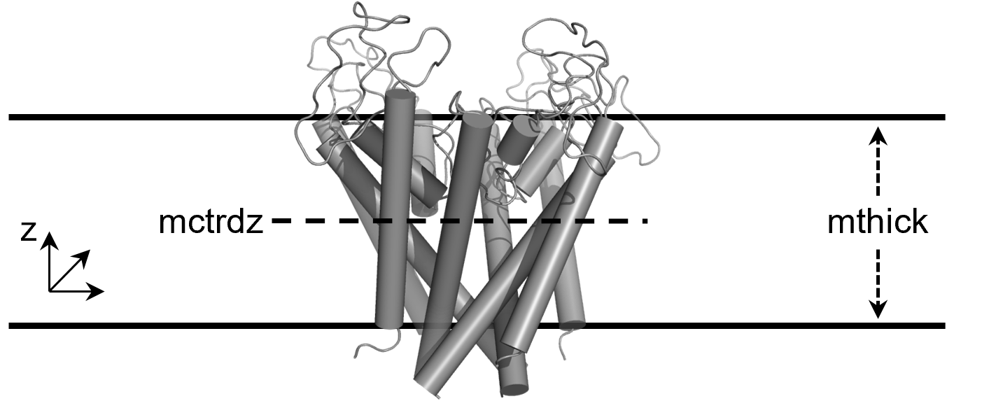
mthick (Default = 40)

Membrane thickness (in Å). This is different from the previous default of 20 Å.

mctrdz (Default = 0.0)

Membrane center (in Å) in the z direction.

poretype (Default = 1)

Turn on and off the automatic depth-first search method to identify the pore. (ref.)

• 0: Do not turn on the pore searching algorithm.
• 1: Turn on the pore searching algorithm.

Options to select numerical procedures¶

npbopt (Default = 0)

Option to select the linear, or the full nonlinear PB equation.

• 0: Linear PB equation (LPBE) is solved
• 1: Nonlinear PB equation (NLPBE) is solved

Note

While the linear PB equation (see tutorial) will suffice for most calculations, the nonlinear PB equation (see tutorial) is recommended for highly charged systems. Parameters such as eneopt or cutnb should be adjusted accordingly when using the NLPBE. Check the following threads (T1 and T2) on how to proceed when using NLPBE. Last but not least, take into account that using NLPBE can significantly increase the calculation time required for PB calculation.

Implemented in v1.5.0

solvopt (Default = 1)

Option to select iterative solvers.

• 1 Modified ICCG or Periodic (PICCG) if bcopt = 10.
• 2 Geometric multigrid. A four-level v-cycle implementation is applied by default.
• 3 Conjugate gradient (Periodic version available under bcopt = 10). This option requires a large linit to converge.
• 4 SOR. This option requires a large linit to converge.
• 5 Adaptive SOR. This is only compatible with npbopt = 1. This option requires a large linit converge. (ref.)
• 6 Damped SOR. This is only compatible with npbopt = 1. This option requires a large linit to converge. (ref.)

accept (Default = 0.001)

Sets the iteration convergence criterion (relative to the initial residue).

Implemented in v1.5.0

linit (Default = 1000)

Sets the maximum number of iterations for the finite difference solvers. Note that linit has to be set to a much larger value, e.g. 10000, for the less efficient solvers, such as conjugate gradient and SOR, to converge. This corresponds to maxitn in pbsa.

fillratio (Default = 4.0)

The ratio between the longest dimension of the rectangular finite-difference grid and that of the solute. For macromolecules is fine to use 4, or a smaller value like 2. A default value of 4 is large enough to be used for a small solute, such as a ligand molecule. Using a smaller value for fillratio may cause part of the small solute to lie outside the finite-difference grid, causing the finite-difference solvers to fail.

scale (Default = 2.0)

Resolution of the Poisson Boltzmann grid. It is equal to the reciprocal of the grid spacing (space in pbsa).

nbuffer (Default = 0)

Sets how far away (in grid units) the boundary of the finite difference grid is away from the solute surface; i.e., automatically set to be at least a solvent probe or ion probe (diameter) away from the solute surface.

Implemented in v1.5.0

nfocus (Default = 2)

Set how many successive FD calculations will be used to perform an electrostatic focussing calculation on a molecule. When nfocus = 1, no focusing is used. It is recommended that nfocus = 1 when the multigrid solver is used.

fscale (Default = 8)

Set the ratio between the coarse and fine grid spacings in an electrostatic focussing calculation.

Implemented in v1.5.0

npbgrid (Default = 1)

Sets how often the finite-difference grid is regenerated.

Implemented in v1.5.0

Options to compute energy and forces¶

bcopt (Default = 5)

Boundary condition options.

• 1: Boundary grid potentials are set as zero, i.e. conductor. Total electrostatic potentials and energy are computed.
• 5: Computation of boundary grid potentials using all grid charges. Total electrostatic potentials and energy are computed.
• 6: Computation of boundary grid potentials using all grid charges. Reaction field potentials and energy are computed with the charge singularity free formalism. (ref.)
• 10: Periodic boundary condition is used. Total electrostatic potentials and energy are computed. Can be used with solvopt = 1, 2, 3, or 4 and ipb = 1 or 2. It should only be used on charge-neutral systems. If the system net charge is detected to be nonzero, it will be neutralized by applying a small neutralizing charge on each grid (i.e. a uniform plasma) before solving.

eneopt (Default = 2)

Option to compute total electrostatic energy and forces.

• 1: Compute total electrostatic energy and forces with the particle-particle particle-mesh (P3M) procedure outlined in Lu and Luo. (ref.) In doing so, energy term EPB in the output file is set to zero, while EEL includes both the reaction field energy and the Coulombic energy. The van der Waals energy is computed along with the particle-particle portion of the Coulombic energy. The electrostatic forces and dielectric boundary forces can also be computed. (ref.) This option requires a nonzero cutnb and bcopt = 5 for soluble proteins / bcopt = 10 for membrane proteins.
• 2: Use dielectric boundary surface charges to compute the reaction field energy. Both the Coulombic energy and the van der Waals energy are computed via summation of pairwise atomic interactions. Energy term EPB in the output file is the reaction field energy. EEL is the Coulombic energy.
• 3: Similar to the first option above, a P3M procedure is applied for both solvation and Coulombic energy and forces for larger systems.
• 4: Similar to the third option above, a P3M procedure for the full nonlinear PB equation is applied for both solvation and Coulombic energy and forces for larger systems. A more robust and clean set of routines were used for the P3M and dielectric surface force calculations.

frcopt (Default = 0)

Option to compute and output electrostatic forces to a file named force.dat in the working directory.

• 0: Do not compute or output atomic and total electrostatic forces.
• 1: Reaction field forces are computed by trilinear interpolation. Dielectric boundary forces are computed using the electric field on dielectric boundary. The forces are output in the unit of kcal/mol·Å.
• 2: Use dielectric boundary surface polarized charges to compute the reaction field forces and dielectric boundary forces (ref.) The forces are output in the unit of kcal/mol·Å.
• 3: Reaction field forces are computed using dielectric boundary polarized charge. Dielectric boundary forces are computed using the electric field on dielectric boundary. (ref.) The forces are output in kcal/mol·Å.

scalec (Default = 0)

Option to compute reaction field energy and forces.

• 0: Do not scale dielectric boundary surface charges before computing reaction field energy and forces.
• 1: Scale dielectric boundary surface charges using Gauss’s law before computing reaction field energy and forces.

Implemented in v1.5.0

cutfd (Default = 5.0)

Atom-based cutoff distance to remove short-range finite-difference interactions, and to add pairwise charge-based interactions. This is used for both energy and force calculations. See Eqn (20) in Lu and Luo. (ref.)

cutnb (Default = 0.0)

Atom-based cutoff distance for van der Waals interactions, and pairwise Coulombic interactions when eneopt = 2. When cutnb is set to the default value of 0, no cutoff will be used for van der Waals and Coulombic interactions, i.e., all pairwise interactions will be included. When eneopt = 1, this is the cutoff distance used for van der Waals interactions only. The particle-particle portion of the Coulombic interactions is computed with the cutoff of cutfd._

nsnba (Default = 1)

Sets how often (steps) atom-based pairlist is generated.

Implemented in v1.5.0

Options to select a non-polar solvation treatment¶

decompopt (Default = 2)

Option to select different decomposition schemes when inp = 2. See (ref.) for a detailed discussion of the different schemes. The σ decomposition scheme is the best of the three schemes studied. (ref.) As discussed in (ref.), decompopt = 1 is not a very accurate approach even if it is more straightforward to understand the decomposition.

• 1: Use the 6/12 decomposition scheme
• 2: Use the σ decomposition scheme
• 3: Use the WCA decomposition scheme

Implemented in v1.5.0

use_rmin (Default = 1)

The option to set up van der Waals radii. The default is to use van der Waals rmin to improve the agreement with TIP3P. (ref.)

• 0: Use atomic van der Waals σ values.
• 1: Use atomic van der Waals rmin values.

Implemented in v1.5.0

sprob (Default = 0.557)

Solvent probe radius (in Å) for solvent accessible surface area (SASA) used to compute the dispersion term, default to 0.557 Å in the σ decomposition scheme as optimized in (ref.) with respect to the TIP3P solvent and the PME treatment. Recommended values for other decomposition schemes can be found in Table 4 of (ref.). If use_sav = 0 (see below), sprob can be used to compute SASA for the cavity term as well. Unfortunately, the recommended value is different from that used in the dispersion term calculation as documented in (ref.). Thus, two separate calculations are needed when use_sav = 0, one for the dispersion term and one for the cavity term. Therefore, please carefully read (ref.) before proceeding with the option of use_sav = 0. Note that sprob was used for ALL three terms of solvation free energies, i.e., electrostatic, attractive, and repulsive terms in previous releases in Amber. However, it was found in the more recent study (ref.) that it was impossible to use the same probe radii for all three terms after each term was calibrated and validated with respect to the TIP3P solvent. (ref.)

Implemented in v1.5.0

vprob (Default = 1.300)

Solvent probe radius (in Å) for molecular volume (the volume enclosed by SASA) used to compute non-polar cavity solvation free energy, default to 1.300 Å, the value optimized in (ref.) with respect to the TIP3P solvent. Recommended values for other decomposition schemes can be found in Tables 1-3 of (ref.).

Implemented in v1.5.0

rhow_effect (Default = 1.129)

Effective water density used in the non-polar dispersion term calculation, default to 1.129 for decompopt = 2, the σ scheme. This was optimized in (ref.) with respect to the TIP3P solvent in PME. Optimized values for other decomposition schemes can be found in Table 4 of (ref.).

Implemented in v1.5.0

use_sav (Default = 1)

The option to use molecular volume (the volume enclosed by SASA) or to use molecular surface (SASA) for cavity term calculation. Recent study shows that the molecular volume approach transfers better from small training molecules to biomacromolecules.

• 0: Use SASA to estimate cavity free energy
• 1: Use the molecular volume enclosed by SASA

Implemented in v1.5.0

cavity_surften (Default = 0.0378)

The regression coefficient for the linear relation between the total non-polar solvation free energy (inp = 1), or the cavity free energy (inp = 2) and SASA/volume enclosed by SASA. The default value is for inp = 2 and set to the best of three tested schemes as reported in (ref.), i.e. decompopt = 2, use_rmin = 1, and use_sav = 1. See recommended values in Tables 1-3 for other schemes.

cavity_offset (Default = -0.5692)

The regression offset for the linear relation between the total non-polar solvation free energy (inp= 1), or the cavity free energy (inp = 2) and SASA/volume enclosed by SASA. The default value is for inp = 2 and set to the best of three tested schemes as reported in (ref.), i.e. decompopt = 2, use_rmin = 1, and use_sav = 1. See recommended values in Tables 1-3 for other schemes.

maxsph (Default = 400)

Approximate number of dots to represent the maximum atomic solvent accessible surface. These dots are first checked against covalently bonded atoms to see whether any of the dots are buried. The exposed dots from the first step are then checked against a non-bonded pair list with a cutoff distance of 9 Å to see whether any of the exposed dots from the first step are buried. The exposed dots of each atom after the second step then represent the solvent accessible portion of the atom and are used to compute the SASA of the atom. The molecular SASA is simply a summation of the atomic SASA’s. A molecular SASA is used for both PB dielectric map assignment and for NP calculations.

Implemented in v1.5.0

maxarcdot (Default = 1500)

Number of dots used to store arc dots per atom.

Options for output¶

npbverb (Default = 0)

Verbose mode.

• 0: Off
• 1: On

Implemented in v1.5.0

&rism namelist variables¶

Closure approximations¶

closure (Default = "kh")

Comma separate list of closure approximations. If more than one closure is provided, the 3D-RISM solver will use the closures in order to obtain a solution for the last closure in the list when no previous solutions are available. The solution for the last closure in the list is used for all output. The use of several closures combined with different tolerances can be useful to overcome convergence issues (see §7.3.1)

• "kh": Kovalenko-Hirata
• "hnc": Hyper-netted chain equation
• "psen": Partial Series Expansion of order-n where “n” is a positive integer (e.g., "pse3")

Examples

=== "v1.5.2"
    === "One closure"
             closure="pse3"
    === "Several closures"
             closure="kh","pse3"
=== "< v1.5.2"
    === "One closure"
             closure="pse3"
    === "Several closures"
             closure="kh,pse3"

Solvation free energy corrections¶

Long-range asymptotics¶

noasympcorr (Default = 1)

Use long-range asymptotic corrections for thermodynamic calculations.

• 0: Do not use long-range corrections
• 1: Use the long-range corrections

Implemented in v1.5.0

treeDCF (Default = 1)

Use direct sum, or the treecode approximation to calculate the direct correlation function long-range asymptotic correction.

• 0: Use direct sum
• 1: Use treecode approximation

Implemented in v1.5.0

treeTCF (Default = 1)

Use direct sum, or the treecode approximation to calculate the total correlation function long-range asymptotic correction.

• 0: Use direct sum
• 1: Use treecode approximation

Implemented in v1.5.0

treeCoulomb (Default = 1)

Use direct sum, or the treecode approximation to calculate the Coulomb potential energy.

• 0: Use direct sum
• 1: Use treecode approximation

Implemented in v1.5.0

treeDCFMAC (Default = 0.1)

Treecode multipole acceptance criterion for the direct correlation function long-range asymptotic correction.

Implemented in v1.5.0

treeTCFMAC (Default = 0.1)

Treecode multipole acceptance criterion for the total correlation function long-range asymptotic correction.

Implemented in v1.5.0

treeCoulombMAC (Default = 0.1)

Treecode multipole acceptance criterion for the Coulomb potential energy.

Implemented in v1.5.0

treeDCFOrder (Default = 2)

Treecode Taylor series order for the direct correlation function long-range asymptotic correction.

Implemented in v1.5.0

treeTCFOrder (Default = 2)

Treecode Taylor series order for the total correlation function long-range asymptotic correction. Note that the Taylor expansion used does not converge exactly to the TCF long-range asymptotic correction, so a very high order will not necessarily increase accuracy.

Implemented in v1.5.0

treeCoulombOrder (Default = 2)

Treecode Taylor series order for the Coulomb potential energy.

Implemented in v1.5.0

treeDCFN0 (Default = 500)

Maximum number of grid points contained within the treecode leaf clusters for the direct correlation function long-range asymptotic correction. This sets the depth of the hierarchical octtree.

Implemented in v1.5.0

treeTCFN0 (Default = 500)

Maximum number of grid points contained within the treecode leaf clusters for the total correlation function long-range asymptotic correction. This sets the depth of the hierarchical octtree.

Implemented in v1.5.0

treeCoulombN0 (Default = 500)

Maximum number of grid points contained within the treecode leaf clusters for the Coulomb potential energy. This sets the depth of the hierarchical octtree.

Implemented in v1.5.0

Solvation box¶

Variable box size¶

buffer (Default = 14)

Minimum distance (in Å) between solute and edge of solvation box. Specify this with grdspc below. Mutually exclusive with ng and solvbox. See §7.2.3 for details on how this affects numerical accuracy and how this interacts with ljTolerance, and tolerance

• when < 0: Use fixed box size (see ng and solvbox below)
• when >= 0: Use buffer distance

grdspc(Default = 0.5,0.5,0.5)

Grid spacing (in Å) of the solvation box. Specify this with buffer above. Mutually exclusive with ng and solvbox.

Fixed box size¶

ng (Default = -1,-1,-1)

Comma separated number of grid points to use in the x, y, and z directions. Used only if buffer < 0. Mutually exclusive with buffer and grdspc above, and paired with solvbox below.

Warning

No default, this must be set if buffer < 0. As a general requirement, the number of grids points in each dimension must be divisible by two, and the number of grid points in the z-axis must be divisible by the number of processes.

As an example: define like ng=1000,1000,1000, where all numbers are divisible by two and you can use 1, 2, 4, 5, 8, 10... pocessors, all divisors of 1000 (value in the z-axis).

Take into account that at a certain level, running RISM in parallel may actually hurt performance, since previous solutions are used as an initial guess for the next frame, hastening convergence. Running in parallel loses this advantage. Also, due to the overhead involved in which each thread is required to load every topology file when calculating energies, parallel scaling will begin to fall off as the number of threads reaches the number of frames.

solvbox (Default = -1,-1,-1)

Sets the size in Å of the fixed size solvation box. Used only if buffer < 0. Mutually exclusive with buffer and grdspc above, and paired with ng above.

Warning

No default, this must be set if buffer < 0. Define like solvbox=20,20,20

solvcut (Default = 14)

Cutoff used for solute-solvent interactions. The default value is that of buffer. Therefore, if you set buffer < 0 and specify ng and solvbox instead, you must set solvcut to a nonzero value; otherwise the program will quit in error.

Solution convergence¶

tolerance (Default = 0.00001)

A comma-separated list of maximum residual values for solution convergence. This has a strong effect on the cost of 3D-RISM calculations (smaller value for tolerance -> more computation). When used in combination with a list of closures it is possible to define different tolerances for each of the closures. This can be useful for difficult to converge calculations (see §7.4.1). For the sake of efficiency, it is best to use as high a tolerance as possible for all but the last closure. See §7.2.3 for details on how this affects numerical accuracy and how this interacts with ljTolerance, buffer, and solvbox. Three formats of list are possible:

• one tolerance: All closures but the last use a tolerance of 1. The last tolerance in the list is used by the last closure. In practice this is the most efficient.
• two tolerances: All closures but the last use the first tolerance in the list. The last tolerance in the list is used by the last closure.
• n tolerances: Tolerances from the list are assigned to the closure list in order.

Examples

v1.5.2<v1.5.2

One closure/One toleranceSeveral closures/One toleranceSeveral closures/Two tolerancesSeveral closures/Several tolerances

closure="pse3", tolerance=0.00001

A tolerance of 0.00001 will be used for clousure "pse3"

 closure="kh","pse3", tolerance=0.00001

A tolerance of 1 will be used for clousure "kh", while 0.00001 will be used for clousure "pse3". Equivalent to closure="kh", "pse3", tolerance=1,0.00001

 closure="kh","pse2","pse3", tolerance=0.01,0.00001

A tolerance of 0.01 will be used for clousures "kh" and "pse2", while 0.00001 will be used for clousure "pse3". Equivalent to closure="kh","pse2","pse3", tolerance=0.01,0.01,0.00001

 closure="kh","pse2","pse3", tolerance=0.1,0.01,0.00001

A tolerance of 0.1 will be used for clousure "kh", 0.01 will be used for clousure "pse2", while 0.00001 will be used for clousure "pse3".

One closure/One toleranceSeveral closures/One toleranceSeveral closures/Two tolerancesSeveral closures/Several tolerances

closure="pse3", tolerance=0.00001

A tolerance of 0.00001 will be used for clousure "pse3"

 closure="kh,pse3", tolerance=0.00001

A tolerance of 1 will be used for clousure "kh", while 0.00001 will be used for clousure "pse3". Equivalent to closure="kh, pse3", tolerance=1,0.00001

 closure="kh,pse2,pse3", tolerance=0.01,0.00001

A tolerance of 0.01 will be used for clousures "kh" and "pse2", while 0.00001 will be used for clousure "pse3". Equivalent to closure="kh,pse2,pse3", tolerance=0.01,0.01,0.00001

 closure="kh,pse2,pse3", tolerance=0.1,0.01,0.00001

A tolerance of 0.1 will be used for clousure "kh", 0.01 will be used for clousure "pse2", while 0.00001 will be used for clousure "pse3".

ljTolerance (Default = -1)

Lennard-Jones accuracy (Optional.) Determines the Lennard-Jones cutoff distance based on the desired accuracy of the calculation. See §7.2.3 for details on how this affects numerical accuracy and how this interacts with tolerance, buffer, and solvbox.

Implemented in v1.5.0

asympKSpaceTolerance (Default = -1)

Tolerance reciprocal space long range asymptotics accuracy (Optional.) Determines the reciprocal space long range asymptotic cutoff distance based on the desired accuracy of the calculation. See §7.2.3 for details on how this affects numerical accuracy. Possible values are:

• when < 0: asympKSpaceTolerance = tolerance/10
• when = 0: no cutoff
• when > 0: given value determines the maximum error in the reciprocal-space long range asymptotics calculations

Implemented in v1.5.0

mdiis_del (Default = 0.7)

MDIIS step size.

Implemented in v1.5.0

mdiis_nvec (Default = 5)

Number of previous iterations MDIIS uses to predict a new solution.

Implemented in v1.5.0

mdiis_restart (Default = 10)

If the current residual is mdiis_restart times larger than the smallest residual in memory, then the MDIIS procedure is restarted using the lowest residual solution stored in memory. Increasing this number can sometimes help convergence.

Implemented in v1.5.0

maxstep (Default = 10000)

Maximum number of iterations allowed to converge on a solution.

Implemented in v1.5.0

npropagate (Default = 5)

Number of previous solutions propagated forward to create an initial guess for this solute atom configuration.

• =0: Do not use any previous solutions
• = 1..5: Values greater than 0 but less than 4 or 5 will use less system memory but may introduce artifacts to the solution (e.g., energy drift).

Implemented in v1.5.0

Output¶

polardecomp (Default = 0)

Decomposes solvation free energy into polar and non-polar components. Note that this typically requires 80% more computation time.

• 0: Do not decompose solvation free energy into polar and non-polar components.
• 1: Decompose solvation free energy into polar and non-polar components.

entropicdecomp (Default = 0)

Decomposes solvation free energy into energy and entropy components. Also performs temperature derivatives of other calculated quantities. Note that this typically requires 80% more computation time and requires a .xvv file version 1.000 or higher (available within GMXMMPBSA data folder). See §7.1.3 and §7.3

• 0: No entropic decomposition
• 1: Entropic decomposition

rism_verbose (Default = 0)

Level of output in temporary RISM output files. May be helpful for debugging or following convergence.

• 0: just print the final result
• 1: additionally prints the total number of iterations for each solution
• 2: additionally prints the residual for each iteration and details of the MDIIS solver (useful for debugging and convergence analyses)

&alanine_scanning namelist variables¶

mutant_res (Default = None. Must be defined)

Define the specific residue that is going to be mutated. Use the following format CHAIN/RESNUM (e.g.: 'A/350') or CHAIN/RESNUM:INSERTION_CODE if applicable (e.g.: "A/27:B").

Important

• Only one residue can be mutated per calculation!
• We recommend using the reference structure (-cr) to ensure the perfect match between the selected residue in the defined structure or topology
• Wehn this varibale is defined, gmx_MMPBSA performs the mutation. This way the user does not have to provide the mutant topology

Changed in v1.4.0: Allows mutation in antibodies since it support insertion code notation

mutant (Default = "ALA")

Defines the residue that it is going to be mutated for. Allowed values are:

• "ALA" or "A": Alanine scanning
• "GLY" or "G": Glycine scanning

Changed in v1.3.0: Change mol (receptor or ligand) by mutant aminoacid (ALA or GLY)

mutant_only (Default = 0)

Option to perform specified calculations only for the mutants.

• 0: Perform calcultion on mutant and original
• 1: Perform calcultion on mutant only

Note

Note that all calculation details are controlled in the other namelists, though for alanine scanning to be performed, the namelist must be included (blank if desired)

cas_intdiel (Default = 0)

The dielectric constant (intdiel(GB)/indi(PB)) will be modified depending on the nature of the residue to be mutated.

• 0: Do not use adaptative intdiel assignation
• 1: Use adaptative intdiel assignation

Important

• Works with the GB and PB calculations
• It is ignored when intdiel(GB)/indi(PB) has been explicitly defined, that is, it is ignored if intdiel != 1.0/indi != 1.0 (default values)
• Dielectric constant values has been assigned according to Yan et al., 2017

Implemented in v1.4.2

intdiel_nonpolar (Default = 1)

Define the intdiel(GB)/indi(PB) value for non-polar residues (PHE, TRP, VAL, ILE, LEU, MET, PRO, CYX, ALA, GLY, PRO)

Implemented in v1.4.2

intdiel_polar (Default = 3)

Define the intdiel(GB)/indi(PB) value for polar residues (TYR, SER, THR, CYM, CYS, HIE, HID, ASN, GLN, ASH, GLH, LYN)

Implemented in v1.4.2

intdiel_positive (Default = 5)

Define the intdiel(GB)/indi(PB) value for positive charged residues (LYS, ARG, HIP)

Implemented in v1.4.2

intdiel_negative (Default = 5)

Define the intdiel(GB)/indi(PB) value for negative charged residues (GLU, ASP)

Implemented in v1.4.2

&decomp namelist variables¶

idecomp

Energy decomposition scheme to use:

• 1: Per-residue decomp with 1-4 terms added to internal potential terms
• 2: Per-residue decomp with 1-4 EEL added to EEL and 1-4 VDW added to VDW potential terms
• 3: Pairwise decomp with 1-4 terms added to internal potential terms
• 4: Pairwise decomp with 1-4 EEL added to EEL and 1-4 VDW added to VDW potential terms

Warning

• No default. This must be specified!

dec_verbose (Default = 0)

Set the level of output to print in the decomp_output file.

• 0: DELTA energy, total contribution only
• 1: DELTA energy, total, sidechain, and backbone contributions
• 2: Complex, Receptor, Ligand, and DELTA energies, total contribution only
• 3: Complex, Receptor, Ligand, and DELTA energies, total, sidechain, and backbone contributions

Note

If the values 0 or 2 are chosen, only the Total contributions are required, so only those will be printed to the mdout files to cut down on the size of the mdout files and the time required to parse them.

print_res (Default = "within 6")

Select residues whose information is going to be printed in the output file. The default selection should be sufficient in most cases, however we have added several additional notations

Selection schemes

By Distance (recommended)Amino acid selectionAll

Notation: [ within distance ]

within corresponds to the keyword and distance to the maximum distance criterion in Å necessary to select the residues from both the receptor and the ligand. In case the cutoff used is so small that the number of decomp residues to print < 2, the cutoff value will be increased by 0.1 until the number of decomp residues to print >= 2.

Example

print_res="within 6" Will print all residues within 6 Å between receptor and ligand including both.

Notation: [ CHAIN/(RESNUM or RESNUM-RESNUM) ]

Print residues individual or ranges. This notation also supports insertion codes, in which case you must define them individually

Example

print_res="A/1,3-10,15,100 B/25" This will print Chain A residues 1, 3 through 10, 15, and 100 along with chain B residue 25 from the complex topology file and the corresponding residues in either the ligand and/or receptor topology files.

Danger

make sure to include at least one residue from both the receptor and ligand in the print_res mask of the &decomp section. Check http://archive.ambermd.org/201308/0075.html

Suppost that we can have the following sequence where chain A is the receptor and B is the ligand: A:LEU:5, A:GLY:6:A, A:THR:6:B, A:SER:6:C A:ASP:6D, A:ILE:7 , B:25

Supported notationWrong notation

Ranges selection

print_res="A/5-7 B/25 Will print all mentioned residues because all residues with insertion code are contained in the range

Individual selection

print_res="A/5,6B,6C,7 B/25 Will print all mentioned residues except the residues 6A and 6D from chain A

print_res="A/5-6B,6D-7 Will end in error.

Notation: all

will print all residues. This option is often not recommended since most residues contribution is zero and it is just going to be a waste of time and computational resources.

Danger

Using idecomp=3 or 4 (pairwise) with a very large number of printed residues and a large number of frames can quickly create very, very large temporary mdout files. Large print selections also demand a large amount of memory to parse the mdout files and write decomposition output file (~500 MB for just 250 residues, since that’s 62500 pairs!) It is not unusual for the output file to take a significant amount of time to print if you have a lot of data. This is most applicable to pairwise decomp, since the amount of data scales as
O(N²).

Important

We recommend using the reference structure (-cr) to ensure the perfect match between the selected residue in the defined structure or topology

Changed in v1.4.0: Improve residue selection

csv_format (Default = 1)

Print the decomposition output in a Comma-Separated-Values (CSV) file. CSV files open natively in most spreadsheets.

• 0: Data to be written out in the standard ASCII format.
• 1: Data to be written out in a CSV file, and standard error of the mean will be calculated and included for all data.

&nmode namelist variables¶

Basic input options¶

nmstartframe²

Frame number to begin performing nmode calculations on

nmendframe² (Default = 1000000)

Frame number to stop performing nmode calculations on

nminterval² (Default = 1)

Offset from which to choose frames to perform nmode calculations on

Parameter options¶

nmode_igb (Default = 1)

Value for Generalized Born model to be used in calculations. Options are:

• 0: Vacuum
• 1: HCT GB model

nmode_istrng (Default = 0.0)

Ionic strength to use in nmode calculations. Units are Molarity (M). Non-zero values are ignored if nmode_igb is 0 above.

dielc (Default = 1.0)

Distance-dependent dielectric constant

drms (Default = 0.001)

Convergence criteria for minimized energy gradient.

maxcyc (Default = 10000)

Maximum number of minimization cycles to use per snapshot in sander.

Sample input files¶

GB¶

 1
 2
 3
 4
 5
 6
 7
 8
 9
10

Sample input file for GB calculation building the Amber topologies
from structures. Please refer to the section "How gmx_MMPBSA works"

&general
startframe=5, endframe=100, interval=5, verbose=2
/

&gb
igb=5, saltcon=0.150,
/

GBNSR6¶

 1
 2
 3
 4
 5
 6
 7
 8
 9
10

Sample input file for GBNSR6 calculation building the Amber topologies
from structures. Please refer to the section "How gmx_MMPBSA works"

&general
startframe=5, endframe=100, interval=5, verbose=2
/

&gbnsr6
epsin=1.0, istrng=0.150,
/

QM/MMGBSA¶

Sample input file for QM/MMGBSA

&general
startframe=5, endframe=100, interval=5,
/

&gb
igb=5, saltcon=0.100, ifqnt=1,
qm_residues="A/240-251 B/297", qm_theory="PM3"
/

PB¶

 1
 2
 3
 4
 5
 6
 7
 8
 9
10

Sample input file for PB calculation building the Amber topologies
from structures. Please refer to the section "How gmx_MMPBSA works"

&general
startframe=5, endframe=100, interval=5
/

&pb
istrng=0.15, fillratio=4.0
/

MMPBSA with membrane proteins¶

Sample input file for MMPBSA with membrane proteins

&general
startframe=1, endframe=100, interval=1,
/

&pb
memopt=1, emem=7.0, indi=4.0,
mctrdz=-10.383, mthick=36.086, poretype=1,
radiopt=0, indi=4.0, istrng=0.150, fillratio=1.25, inp=2,
sasopt=0, solvopt=2, ipb=1, bcopt=10, nfocus=1, linit=1000,
eneopt=1, cutfd=7.0, cutnb=99.0,
maxarcdot=15000,
npbverb=1,
/

MM/3D-RISM¶

Sample input file for 3D-RISM

&general
startframe=20, endframe=100, interval=5,
/

&rism
polardecomp=1, thermo="gf"
/

Alanine scanning¶

 1
 2
 3
 4
 5
 6
 7
 8
 9
10
11
12
13

Sample input file for Alanine scanning

&general
startframe=5, endframe=21, interval=1, PBRadii=4
/

&gb
igb=8, saltcon=0.150, intdiel=10
/

&alanine_scanning
mutant='ALA', mutant_res='B:12'
/

Decomposition analysis¶

Sample input file for decomposition analysis
Make sure to include at least one residue from both the receptor
and ligand in the print_res mask of the &decomp section.
http://archive.ambermd.org/201308/0075.html. This is automally
guaranteed when using "within" keyword.

&general
startframe=5, endframe=21, interval=1,
/

&gb
igb=5, saltcon=0.150,
/

&decomp
idecomp=2, dec_verbose=3,
# This will print all residues that are less than 4 Å between
# the receptor and the ligand
print_res="within 4"
/

Entropy with NMODE¶

 1
 2
 3
 4
 5
 6
 7
 8
 9
10
11
12
13
14
15

Sample input file for entropy calculations

&general
startframe=5, endframe=21, interval=1,
temperature=298
/

&gb
igb=2, saltcon=0.150,
/

&nmode
nmstartframe=10, nmendframe=21, nminterval=2,
maxcyc=50000, drms=0.0001,
/

Interaction Entropy¶

 1
 2
 3
 4
 5
 6
 7
 8
 9
10
11
12
13

Sample input file for entropy calculations

&general
startframe=5, endframe=21, interval=1,
# Interaction Entropy (IE)
# (https://pubs.acs.org/doi/abs/10.1021/jacs.6b02682) approximation
forcefields="oldff/leaprc.ff99SB", interaction_entropy=1, ie_segment=25,
temperature=298
/

&gb
igb=2, saltcon=0.150,
/