Introduction¶

MM/PB(GB)SA method can be used for calculating binding free energies of non covalently bound complexes.

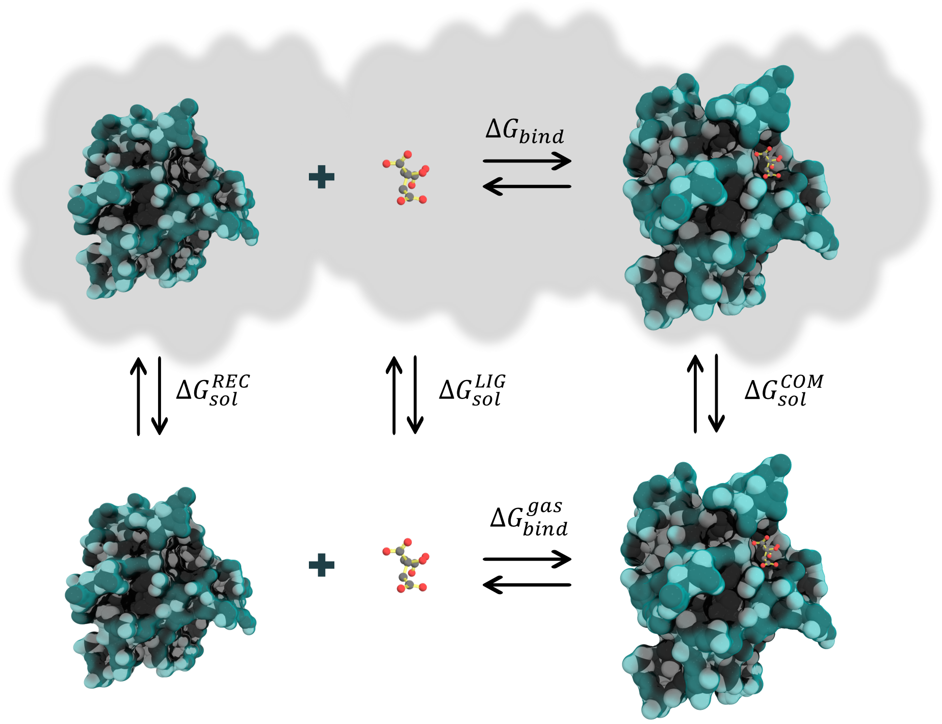
drawing — **Figure 1.** Thermodynamic cycle for binding free energy calculations

The free binding energy for a complex can be estimated as follows:

∆𝐺_{𝑏𝑖𝑛𝑑} = 〈𝐺_𝐶𝑂𝑀〉−〈𝐺_𝑅𝐸𝐶〉−〈𝐺_𝐿𝐼𝐺〉

(1)

where each term to the right in the equation is given by:

〈𝐺_𝑥〉 = 〈𝐸_𝑀𝑀〉 + 〈𝐺_𝑠𝑜𝑙〉 − 〈𝑇𝑆〉

(2)

In turn, ∆𝐺_{𝑏𝑖𝑛𝑑} can also be represented as:

∆𝐺_{𝑏𝑖𝑛𝑑} = ∆𝐻 − 𝑇∆𝑆

(3)

where ∆𝐻 corresponds to the enthalpy of binding and −𝑇∆𝑆 to the conformational entropy after ligand binding. When the entropic term is dismissed, the computed value is the effective free energy, which is usually sufficient for comparing relative binding free energies of related ligands.

The ∆𝐻 can be decomposed into different terms:

∆𝐻 = ∆𝐸_𝑀𝑀 + ∆𝐺_𝑠𝑜𝑙

(4)

where:

∆𝐸_𝑀𝑀 = ∆𝐸_{𝑏𝑜𝑛𝑑𝑒𝑑} + ∆𝐸_{𝑛𝑜𝑛𝑏𝑜𝑛𝑑𝑒𝑑} = (∆𝐸_{𝑏𝑜𝑛𝑑} + ∆𝐸_{𝑎𝑛𝑔𝑙𝑒} + ∆𝐸_{𝑑𝑖ℎ𝑒𝑑𝑟𝑎𝑙}) + (∆𝐸_𝑒𝑙𝑒 + ∆𝐸_𝑣𝑑𝑊)

(5)

The gas phase free energy contributions (∆𝐸_𝑀𝑀) are calculated by sander within the AmberTools package according to the force field used in the MD simulation.

The ∆𝐺_𝑠𝑜𝑙 is given by:

∆𝐺_𝑠𝑜𝑙 = ∆𝐺_𝑝𝑜𝑙 + ∆𝐺_{𝑛𝑜𝑛−𝑝𝑜𝑙} = ∆𝐺_{𝑃𝐵/𝐺𝐵} + ∆𝐺_{𝑛𝑜𝑛−𝑝𝑜𝑙}

(6)

where:

∆𝐺_{𝑛𝑜𝑛−𝑝𝑜𝑙𝑎𝑟} = 𝑁𝑃_{𝑇𝐸𝑁𝑆𝐼𝑂𝑁} ∗ ∆𝑆𝐴𝑆𝐴 + 𝑁𝑃_{𝑂𝐹𝐹𝑆𝐸𝑇}

(7)

or,

∆𝐺_{𝑛𝑜𝑛−𝑝𝑜𝑙} = ∆𝐺_{𝑑𝑖𝑠𝑝} + ∆𝐺_{𝑐𝑎𝑣𝑖𝑡𝑦} = ∆𝐺_{𝑑𝑖𝑠𝑝} + (𝐶𝐴𝑉𝐼𝑇𝑌_{𝑇𝐸𝑁𝑆𝐼𝑂𝑁} ∗ ∆𝑆𝐴𝑆𝐴 + 𝐶𝐴𝑉𝐼𝑇𝑌_{𝑂𝐹𝐹𝑆𝐸𝑇})

(8)

In the above equations, ∆𝐸_𝑀𝑀 corresponds to the molecular mechanical energy changes in the gas phase. ∆𝐸_𝑀𝑀 includes ∆𝐸_{𝑏𝑜𝑛𝑑𝑒𝑑}, also known as internal energy, and ∆𝐸_{𝑛𝑜𝑛𝑏𝑜𝑛𝑑𝑒𝑑}, corresponding to the van der Waals and electrostatic contributions. The solvation energy is determined differently, depending on the method employed. In the 3D-RISM model, both components -polar and non-polar- of the solvation energy are calculated. However, the PB and GB models estimate only the polar component of the solvation. The non-polar component is usually assumed to be proportional to the molecule's total solvent accessible surface area (SASA), with a proportionality constant derived from experimental solvation energies of small non-polar molecules (eq. 7). Alternatively, a modern approach that separates non-polar solvation free energies into cavity and dispersion terms can be used. In this approach, SASA is used to correlate the cavity term only, while a surface-integration method is employed to compute the dispersion term (eq. 8).

Furthermore, the entropic component is usually calculated by normal modes analysis (NMODE). The translational and rotational entropies can be estimated using standard statistical mechanical formulas. Nevertheless, calculating vibrational entropy using normal modes is computationally expensive because it requires expanding the internal coordinate covariance matrix for all degrees of freedom for a set of minimized structures. Conversely, the Quasi-harmonic (QH) approximation is less computationally expensive, although it requires a considerable number of frames to converge. Recently, other alternatives have been developed, such as NMODE in truncated systems, which considerably reduces the computational cost. Interaction Entropy (IE) is another novel method that calculates the entropic component of the binding free energy directly from MD simulations without any extra computational cost. This method is numerically reliable, more computationally efficient, and superior to the standard NMODE approach, as shown in an extensive study of over a dozen randomly selected protein-ligand binding systems.

Typically, two approaches are used for MM/PB(GB)SA calculations, known as Single Trajectory Protocol (STP) and Multiple Trajectory Protocol (MTP). In STP, both the receptor and the ligand trajectories are extracted from that of the complex. This approach is valid when the bound and unbound states of the receptor, and the ligand are similar. It is computationally less expensive than the MTP approach since only a simulation of the complex is required. Additionally, the potential internal terms (e.g., bonds, angles, and dihedrals) cancel exactly in STP since these terms are the same in both bound and unbound states. On the other hand, the MTP is a more realistic approach because it considers multiple trajectories (i.e., complex, receptor, and ligand). However, significant conformational changes can lead to numerous errors. In practice, a detailed study of the system is required to select the approach to be used.

Literature¶

Further information can be found in Amber manual:

and the foundational papers:

as well as some reviews and expert opinions:

Last update: February 26, 2022 03:38:16
Created: February 8, 2021 07:10:13